Transformer
> The Transformer is a deep learning model introduced in 2017 that utilizes the mechanism of attention. It is used primarily in the field of natural language processing (NLP), but recent research has also developed its application in other tasks like video understanding. Wikipedia
In this document we will see how to implement an equivariant attention mechanism with e3nn.
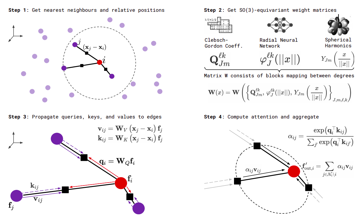
We will implement the formula (1) of SE(3)-Transformers. The output features \(f'\) are computed by
where \(q, k, v\) are respectively called the queries, keys and values. They are functions of the input features \(f\).
all these formula are well illustrated by the figure (2) of the same article.
First we need to define the irreps of the inputs, the queries, the keys and the outputs. Note that outputs and values share the same irreps.
# Just define arbitrary irreps
irreps_input = o3.Irreps("10x0e + 5x1o + 2x2e")
irreps_query = o3.Irreps("11x0e + 4x1o")
irreps_key = o3.Irreps("12x0e + 3x1o")
irreps_output = o3.Irreps("14x0e + 6x1o")  # also irreps of the values
Lets create a random graph on which we can apply the attention mechanism:
num_nodes = 20

pos = torch.randn(num_nodes, 3)
f = irreps_input.randn(num_nodes, -1)

# create graph
max_radius = 1.3
edge_src, edge_dst = radius_graph(pos, max_radius)
edge_vec = pos[edge_src] - pos[edge_dst]
edge_length = edge_vec.norm(dim=1)
The queries \(q_i\) are a linear combination of the input features \(f_i\).
h_q = o3.Linear(irreps_input, irreps_query)
In order to generate weights that depends on the radii, we project the edges length on a basis:
number_of_basis = 10
edge_length_embedded = soft_one_hot_linspace(
    edge_length,
    start=0.0,
    end=max_radius,
    number=number_of_basis,
    basis='smooth_finite',
    cutoff=True  # goes (smoothly) to zero at `start` and `end`
)
edge_length_embedded = edge_length_embedded.mul(number_of_basis**0.5)
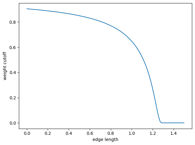
We will also need a number between 0 and 1 that indicates smoothly if the length of the edge is smaller than max_radius.
edge_weight_cutoff = soft_unit_step(10 * (1 - edge_length / max_radius))
Here is a figure of the function used:
To create the values and the keys we have to use the relative position of the edges. We will use the spherical harmonics to have a richer describtor of the relative positions:
irreps_sh = o3.Irreps.spherical_harmonics(3)
edge_sh = o3.spherical_harmonics(irreps_sh, edge_vec, True, normalization='component')
We will make a tensor prodcut between the input and the spherical harmonics to create the values and keys. Because we want the weights of these tensor products to depend on the edge length we will generate the weights using multi layer perceptrons.
tp_k = o3.FullyConnectedTensorProduct(irreps_input, irreps_sh, irreps_key, shared_weights=False)
fc_k = nn.FullyConnectedNet([number_of_basis, 16, tp_k.weight_numel], act=torch.nn.functional.silu)

tp_v = o3.FullyConnectedTensorProduct(irreps_input, irreps_sh, irreps_output, shared_weights=False)
fc_v = nn.FullyConnectedNet([number_of_basis, 16, tp_v.weight_numel], act=torch.nn.functional.silu)
For the correpondance with the formula, tp_v, fc_v represent \(h_K\) and tp_v, fc_v represent \(h_V\).
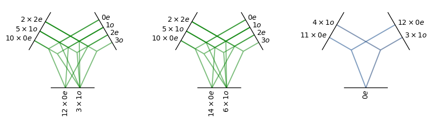
Then we need a way to compute the dot product between the queries and the keys:
dot = o3.FullyConnectedTensorProduct(irreps_query, irreps_key, "0e")
The operations tp_k, tp_v and dot can be visualized as follow:
Finally we can just use all the modules we created to compute the attention mechanism:
# compute the queries (per node), keys (per edge) and values (per edge)
q = h_q(f)
k = tp_k(f[edge_src], edge_sh, fc_k(edge_length_embedded))
v = tp_v(f[edge_src], edge_sh, fc_v(edge_length_embedded))

# compute the softmax (per edge)
exp = edge_weight_cutoff[:, None] * dot(q[edge_dst], k).exp()  # compute the numerator
z = scatter(exp, edge_dst, dim=0, dim_size=len(f))  # compute the denominator (per nodes)
z[z == 0] = 1  # to avoid 0/0 when all the neighbors are exactly at the cutoff
alpha = exp / z[edge_dst]

# compute the outputs (per node)
f_out = scatter(alpha.relu().sqrt() * v, edge_dst, dim=0, dim_size=len(f))
Note that this implementation has small differences with the article.
Special care was taken to make the whole operation smooth when we move the points (deleting/creating new edges). It was done via
edge_weight_cutoff,edge_length_embeddedand the property \(f(0)=0\) for the radial neural network.The output is weighted with \(\sqrt{\alpha_{ij}}\) instead of \(\alpha_{ij}\) to ensure a proper normalization.
Both are checked below, starting by the normalization.
f_out.mean().item(), f_out.std().item()
(-0.10737190395593643, 1.2174392938613892)
Let’s put eveything into a function to check the smoothness and the equivariance.
def transformer(f, pos):
    edge_src, edge_dst = radius_graph(pos, max_radius)
    edge_vec = pos[edge_src] - pos[edge_dst]
    edge_length = edge_vec.norm(dim=1)

    edge_length_embedded = soft_one_hot_linspace(
        edge_length,
        start=0.0,
        end=max_radius,
        number=number_of_basis,
        basis='smooth_finite',
        cutoff=True
    )
    edge_length_embedded = edge_length_embedded.mul(number_of_basis**0.5)
    edge_weight_cutoff = soft_unit_step(10 * (1 - edge_length / max_radius))

    edge_sh = o3.spherical_harmonics(irreps_sh, edge_vec, True, normalization='component')

    q = h_q(f)
    k = tp_k(f[edge_src], edge_sh, fc_k(edge_length_embedded))
    v = tp_v(f[edge_src], edge_sh, fc_v(edge_length_embedded))

    exp = edge_weight_cutoff[:, None] * dot(q[edge_dst], k).exp()
    z = scatter(exp, edge_dst, dim=0, dim_size=len(f))
    z[z == 0] = 1
    alpha = exp / z[edge_dst]

    return scatter(alpha.relu().sqrt() * v, edge_dst, dim=0, dim_size=len(f))
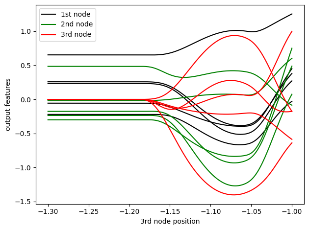
Here is a smoothness check: tow nodes are placed at a distance 1 (max_radius > 1) so they see each other.
A third node coming from far away moves slowly towards them.
f = irreps_input.randn(3, -1)

xs = torch.linspace(-1.3, -1.0, 200)
outputs = []

for x in xs:
    pos = torch.tensor([
        [0.0, 0.5, 0.0],       # this node always sees...
        [0.0, -0.5, 0.0],      # ...this node
        [x.item(), 0.0, 0.0],  # this node moves slowly
    ])

    with torch.no_grad():
        outputs.append(transformer(f, pos))

outputs = torch.stack(outputs)
plt.plot(xs, outputs[:, 0, [0, 1, 14, 15, 16]], 'k')  # plots 2 scalars and 1 vector
plt.plot(xs, outputs[:, 1, [0, 1, 14, 15, 16]], 'g')
plt.plot(xs, outputs[:, 2, [0, 1, 14, 15, 16]], 'r')
Finally we can check the equivariance:
f = irreps_input.randn(10, -1)
pos = torch.randn(10, 3)

rot = o3.rand_matrix()
D_in = irreps_input.D_from_matrix(rot)
D_out = irreps_output.D_from_matrix(rot)

f_before = transformer(f @ D_in.T, pos @ rot.T)
f_after = transformer(f, pos) @ D_out.T

torch.allclose(f_before, f_after, atol=1e-3, rtol=1e-3)
True
Extra sanity check of the backward pass:
for x in [0.0, 1e-6,  max_radius / 2, max_radius - 1e-6, max_radius, max_radius + 1e-6, 2 * max_radius]:
    f = irreps_input.randn(2, -1, requires_grad=True)
    pos = torch.tensor([
        [0.0, 0.0, 0.0],
        [x, 0.0, 0.0],
    ], requires_grad=True)
    transformer(f, pos).sum().backward()

    assert f.grad is None or torch.isfinite(f.grad).all()
    assert torch.isfinite(pos.grad).all()